Example 2.2

Pade Differentiation Using a Lower Order Boundry Scheme

Contents

Setup
Construct difference scheme
Compute approximate derivative
Generate Plots

Setup

close all;
clear f df N H h func deriv A b i approx_deriv;

% function and derivative
f = @(x) sin(5*x);
df = @(x) 5*cos(5*x);

% grid
N = 15;
H = linspace(0,3,N);
h = 3/(N-1);

% sample function and derivative
func = f(H)';
deriv = df(H)';

Construct difference scheme

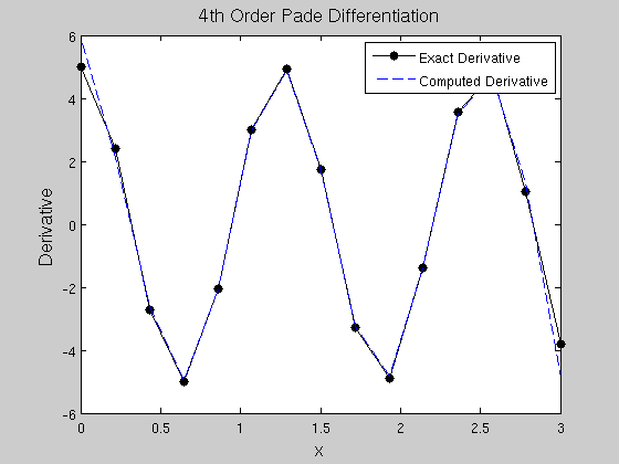
Here we are using a fourth-order Pade scheme with third order boundary schemes given by (2.17) in the text.

A = zeros(N,N);
b = zeros(N,1);
A(1,1:2) = [1 2];
A(N,N-1:N) = [2 1];
b(1) = -5*func(1)/2 + 2*func(2) + func(3)/2;
b(N) = 5*func(N)/2 - 2*func(N-1) - func(N-2)/2;
for i = 2:N-1
    A(i,i-1:i+1) = [1 4 1];
    b(i) = 3*(func(i+1)-func(i-1));
end
b = b/h;

Compute approximate derivative

approx_deriv = A\b;

Generate Plots

figure(1);clf
plot(H,deriv,'k.-','MarkerSize',20)
hold on
plot(H,approx_deriv,'--')
xlabel('x','Fontsize',14)
ylabel('Derivative','Fontsize',14)
title('4th Order Pade Differentiation','Fontsize',14)
legend('Exact Derivative','Computed Derivative')