Example 4.7

Multi-Step Methods Same problem as example 4.3

Contents

Setup

close all;
clear h w Tmax N t g T y_true f Ylf i Yab;

h = 0.1;
w = 4;
Tmax = 6;
N = Tmax / h;
t = linspace(0,6,N+1);

Analyic solution

g = @(x) cos(w*x);
T = linspace(0,6,100);
y_true = g(T);

Function

f = @(t,y) [y(2); -16*y(1)];

Leapfrog

initial values

Ylf = [1; 0];
% take first step
Ylf(:,2) = Ylf(:,1) + h*f(t(1),Ylf(:,1));
% take remaining leapfrog steps
for i=2:N
    Ylf(:,i+1) = Ylf(:,i-1) + 2*h*f(t(i),Ylf(:,i));
end

Adams-Bashforth

initial values

Yab = [1; 0];
% take first step
Yab(:,2) = Yab(:,1) + h*f(t(1),Yab(:,1));
% take remaining leapfrog steps
for i=2:N
    Yab(:,i+1) = Yab(:,i) + 3/2*h*f(t(i),Yab(:,i)) - h/2*f(t(i-1),Yab(:,i-1));
end

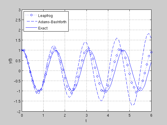
Plot Generation

figure(1); clf
plot(t,Ylf(1,:),'o:')
hold on
plot(t,Yab(1,:),'--')
plot(T,y_true)
axis([0 6 -2 3])
grid on
legend('Leapfrog','Adams-Bashforth','Exact','Location','NorthWest')
xlabel('t')
ylabel('y(t)')

Published with MATLAB® 7.5