Example 5.6

Approximate Factorization for the Heat Equation

This example uses matlab sparse matrices as the operators. This makes the code short and clean. But, care must be taken in applying the correct operator to the correct data. Matlab's meshgrid function stores x-values horizontally and y-values vertically in the data. When applying a matrix operator to data you are operating on the columns.

For example, say T is the data array. Ay is an operator on y-data and Ax is an operator on x-data. The application must be done in this way: Ay*T - to operate on the y-data Ax*T' - data must be transposed before applying the x operator

Note 1: An alternative to this method would be to store all of the data in a 1-dimensional array. However, this complicates the construction of the operators and plotting in matlab.

Note 2: Comments in this code use the following terms y-major: when y-data is organized in columns, the defualt state x-major: when x-data is organized in columns, usually after a transpose

Contents

Set up

close all;

M = 20;  % points in the x direction
N = 20;  % points in the y direction

x0 = -1;
xM = 1;
y0 = -1;
yN = 1;

dx = (xM-x0)/M;
dy = (yN-y0)/N;

x = linspace(x0,xM,M+1);
y = linspace(y0,yN,N+1);

[X Y] = meshgrid(x,y);

q = 2*(2-X.^2 - Y.^2);

operators

Ax = 1/(dx^2).*gallery('tridiag',M-1,1,-2,1);
Ay = 1/(dy^2).*gallery('tridiag',N-1,1,-2,1);
Ix = speye(M-1);
Iy = speye(N-1);

Time advancement 1

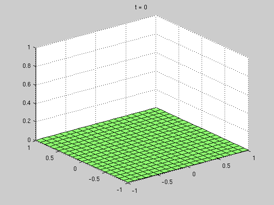
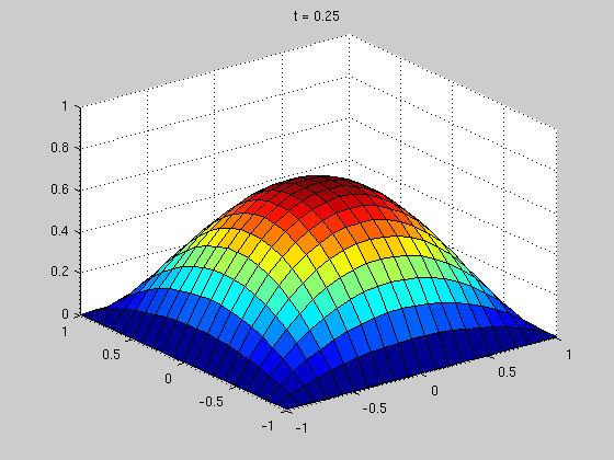
dt = 0.05;             % time step
T = zeros(N+1,M+1);    % initial condition

t_final = 1.0;         % final time
time = 0:dt:t_final;   % time array
pt = [0.0 0.25 1.0];   % desired plot times
pn = length(pt);       % number of desired plots
pc = 1;                % plot counter
rt = zeros(1,pn);      % actual plot times
S = zeros(N+1,M+1,pn); % solution storage

for t = time
    % plot storage
    if ( t >= pt(pc) )
        S(:,:,pc) = T;
        rt(pc) = t;
        pc = pc + 1;
        if (pc > pn)
            break
        end
    end

    r1 = (Iy + dt/2*Ay) * T(2:N,2:M);  % r1 is y-major
    r2 = (Ix + dt/2*Ax) * r1';         % r2 is x-major
    r = r2 + dt*q(2:N,2:M)';           % r is x-major

    T1 = (Ix - dt/2*Ax) \ r;           % T1 is x-major
    T(2:N,2:M) = (Iy - dt/2*Ay) \ T1'; % T is y-major

end

Plot

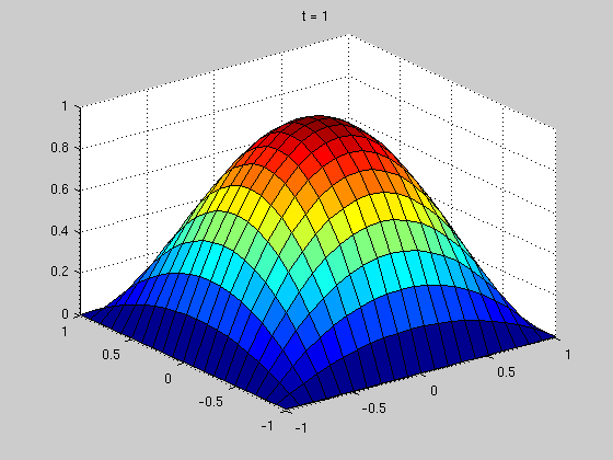
figure(1);
surf(X,Y,S(:,:,1))
zlim([0 1])
title(['t = ' num2str(rt(1))])

figure(2)
surf(X,Y,S(:,:,2))
zlim([0 1])
title(['t = ' num2str(rt(2))])

figure(3)
surf(X,Y,S(:,:,3))
zlim([0 1])
title(['t = ' num2str(rt(3))])

Compute error

% true solution
P = (X.^2 - 1).*(Y.^2 - 1);

% max pointwise difference
mpd1 = max(max(abs(P-S(:,:,3))))

% max pointwise percentage
mpp1 = max(max(abs(P(2:N,2:M)-S(2:N,2:M,3))./P(2:N,2:M)))

% percentage error volume
pev1 = sum(sum(abs(P-S(:,:,3))))/sum(sum(P))

mpd1 =

   0.007690179217719


mpp1 =

   0.007690179217719


pev1 =

   0.007018872300514

Time advancement 2

dt = 1;                % time step
T = zeros(N+1,M+1);    % initial condition

t_final = 5.0;         % final time
time = 0:dt:t_final;   % time array
pt = [5.0];            % desired plot times
pn = length(pt);       % number of desired plots
pc = 1;                % plot counter
rt = zeros(1,pn);      % actual plot times
S = zeros(N+1,M+1,pn); % solution storage

for t = time
    % plot storage
    if ( t >= pt(pc) )
        S(:,:,pc) = T;
        rt(pc) = t;
        pc = pc + 1;
        if (pc > pn)
            break
        end
    end

    r1 = (Iy + dt/2*Ay) * T(2:N,2:M);  % r1 is y-major
    r2 = (Ix + dt/2*Ax) * r1';         % r2 is x-major
    r = r2 + dt*q(2:N,2:M)';           % r is x-major

    T1 = (Ix - dt/2*Ax) \ r;           % T1 is x-major
    T(2:N,2:M) = (Iy - dt/2*Ay) \ T1'; % T is y-major

end

Compute error

% true solution
P = (X.^2 - 1).*(Y.^2 - 1);

% max pointwise difference
mpd2 = max(max(abs(P-S(:,:,1))))

% max pointwise percentage
mpp2 = max(max(abs(P(2:N,2:M)-S(2:N,2:M,1))./P(2:N,2:M)))

% percentage error volume
pev2 = sum(sum(abs(P-S(:,:,1))))/sum(sum(P))

mpd2 =

     3.885037657249679e-04


mpp2 =

   0.006858024743513


pev2 =

     2.241660343727758e-04

Published with MATLAB® 7.5