Example 6.7

Initial Boundary Value Problem

Contents

Initialization

close all;
clear N dX X u_0 k uk_0 uk2 u fun time soln
clear uk_sol u_sol h


N = 32;
dX = 1/N;

X = [0:dX:1-dX]';

Initial Conditions

u_0 = zeros(N,1);
for j = [1:length(X)]
    if X(j)<0.4
        u_0(j) = 1-25*(X(j)-0.2)^2;
    end;
end;

Solve the ODE

k     = 2*pi*[0:N/2-1]';
uk_0  = fft(u_0)/N;
uk_0  = uk_0(1:N/2,1);

uk2 = [uk_0;0;conj(flipud(uk_0(2:N/2)))];
u = ifft(uk2*N);

fun = @(t,u) -(i*k + 0.05*k.^2).*u;

[time,soln] = ode45(fun,[0:0.006:0.75],uk_0);

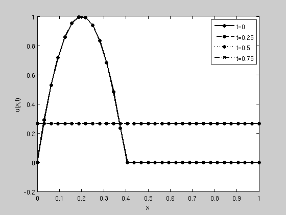
Plot the solution (figure 6.9)

uk_sol = zeros(N/2,1,3);
u_sol  = zeros(N,1,3);
uk_sol(:,:,1) = soln(42,:).';
uk_sol(:,:,2) = soln(83,:).';
uk_sol(:,:,3) = soln(125,:).';

for k = [1:3]
    uk = [uk_sol(:,:,k);0;conj(flipud(uk_sol(2:N/2,1,k)))];
    u_sol(:,:,k) = ifft(uk*N);
end;

figure;
plot([X;X(N)+dX],[u_0;u_0(1)],'k-o',...
     'LineWidth',2,'MarkerFaceColor','k');
hold on;
plot([X;X(N)+dX],[u_sol(:,1,1);u_sol(1,1,1)],'k--o',...
     'LineWidth',2,'MarkerFaceColor','k');
plot([X;X(N)+dX],[u_sol(:,1,2);u_sol(1,1,2)],'k:o',...
     'LineWidth',2,'MarkerFaceColor','k');
plot([X;X(N)+dX],[u_sol(:,1,3);u_sol(1,1,3)],'k-.x',...
     'LineWidth',2,'MarkerFaceColor','k');
xlabel('x');ylabel('u(x,t)');

legend('t=0',...
       't=0.25',...
       't=0.5',...
       't=0.75');

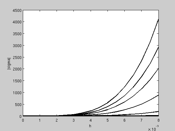
Reproduce figure 6.8

figure;
h = [0:5e-4:8e-3];
for n = [1,5,8,11,13,14,15]
    k = 2*pi*n;
    lambda = -(i*k+0.05*k^2);
    lh = lambda * h;

    sigma = abs(1 + lh + (lh.^2)/2 + (lh.^3)/6 + (lh.^4)/24);
    plot(h,sigma,'k','LineWidth',2);
    xlabel('h'); ylabel('|sigma|');
    hold on;
end;

Published with MATLAB® 7.5