Example 4.9

Shooting to Solve the Blasius Boundary Layer: f''' + f*f'' = 0

Contents

Clean and Setup
Function
Initial Solves
Shooting
Generate Plots

Clean and Setup

close all;
clear N iter f t y1 y2 f1a f1b f2a f2b y;

N = 1000;
iter = 8;

Function

f = @(t,y) [-y(1)*y(3); y(1); y(2)];

Initial Solves

[t y1] = rk4(f,[0 10],[1 0 0],N);
[t y2] = rk4(f,[0 10],[.5 0 0],N);
f1a = .5;
f1b = 1;
f2a = y2(2,end);
f2b = y1(2,end);

Shooting

tol = 1e-18;
for i = 1:iter
    f1new = f1a + (f1a-f1b)/(f2a-f2b)*(1-f2a);
    [t y] = rk4(f,[0 10],[f1new 0 0],N);
    fprintf('iter:%2d, f1(0)=%17.15f, f2(10)=%17.15f\n',i,f1new,y(2,end));
    if ( abs(y(2,end)-1) <= tol )
        break;
    end
    f1b = f1a;
    f1a = f1new;
    f2b = f2a;
    f2a = y(2,end);
end

iter: 1, f1(0)=0.465138301848175, f2(10)=0.993655903270372
iter: 2, f1(0)=0.469647413264798, f2(10)=1.000067325527485
iter: 3, f1(0)=0.469600063660851, f2(10)=1.000000106891883
iter: 4, f1(0)=0.469599988364941, f2(10)=0.999999999998203
iter: 5, f1(0)=0.469599988366207, f2(10)=0.999999999999999
iter: 6, f1(0)=0.469599988366207, f2(10)=1.000000000000000

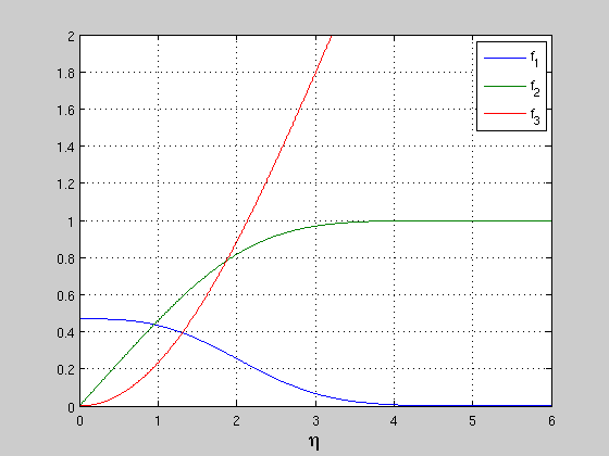
Generate Plots

plot(t,y)
grid on
axis([0 6 0 2])
legend('f_1','f_2','f_3')
xlabel('\eta','FontSize',14)